When integrations or differentiations are carried out they are at the resolution rc. The details of the interpolation methods (such as methods of rounding used) have been carefully chosen to give the expected results and variation from the analytical values are rarely more than a single year with the standard options.
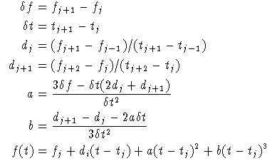
The files for the calibration curve usually have a different resolution to the internal storage resolution and so some form of interpolation is needed. This can either be linear or a cubic function depending on the setting in the system options. The cubic interpolation does not fit a spline function as this is very time consuming to calculate and can have some undesirable features such as large excursions between points. The cubic function used here gives a smooth curve with a continuous first differential but gives very little overall difference from the linear interpolation. The form of the function between two points is simply defined by the four surrounding points. If fj defines the function at tj the interpolation between tj and tj+1 is given by f(t) where:
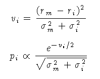
The calibration curve is stored in two arrays one ri defining the radiocarbon age of the tree rings and another sigmai defining the errors associated with these measurements. Both ri and sigmai which are stored at the resolution rs are generated from the supplied calibration curves using the above interpolation method.
yCAL = 1950 - yBP
Thus:
10BP = 1940AD, 11950BP = 10000BC
It should be noted that this does imply a year 0 in the AD/BC sequence which is strictly speaking incorrect. With radiocarbon dates the problem is clearly semantic, with historical evidence it should be borne in mind that age differences across the BC/AD boundary are actually one year larger that they should be. Alternatively negative numbers (BC) should always be taken as the start of the year and positive numbers (AD) as the end. Thus -1 is the start of the first year BC whereas +1 is the end of the year 1AD. The reason for this problem is that in order to keep the internal representation of the numbers consistent it is very difficult to have to deal with a number set which goes from -1 to 1.
In this program the distribution is left normalised to a maximum of 1 rather than the actual probability of any individual year.
NOTE This is different to old versions of OxCal (pre 3.2) where pi was simply set to exp(-vi/2).
See also [Archaeological Considerations]

Solution of this differential equation requires a knowledge of the curve R(t) for all times before t. A linear extrapolation is assumed before the start of the curve using a gradient estimated from the first half of the curve R(t). The uncertainties in this are assumed to be ten times larger than those quoted for the first point in the curve; in practice these assumptions are unlikely to be significant unless the time constant is very long or you are considering points close to the start of the calibration curve.
Treatment of the uncertainties is more complicated. If the uncertainties associated with each point on the calibration curve are assumed to be independent the uncertainties in the reservoir curve should be smaller. In practice the errors almost certainly to some extent systematic. They have therefore been treated in exactly the same way as the concentrations themselves: if sigma(t) and Sigma(t) are the respective uncertainties we assume:

If there are also uncertainties in tau the solution of the equations would involve a double integration which would in practice be very slow. Another algorithm has therefore been adopted which is to increase the sigma in proportion to the difference between R(t) and r(t). Thus if the uncertainty in tau is deltatau:

For the oceans a properly modeled ocean curve should be used (see Stuiver et al 1998 - marine data). Local corrections can then be made using a Delta_R correction term:

See also [Calibration Data]
and the proportion of the second curve is P � D then the resultant distribution is given by:
See also [Calibration Data]
tc = tm - (dm/dr)
dtc = -(ddm/dr)
Rounding to the nearest rc will take place at this stage so you may notice a slight change in the entered values especially if rc is 10 or 100.
Calculation of symmetric probability distributions is simple:

The function used for asymmetric dates is rather more complex:

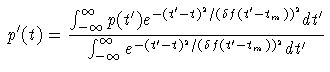
p'(t) = p(t/f)
And a proportional error df by using the mapping:
The distribution is then renormalised.
In the program these error factors are normally calculated before each distribution is reported except in the case of functions such as Combine which give a resultant distribution when the factor is only applied to the final result to prevent the systematic errors being reduced in the combination process.
The probability method (selected for all types of distribution in the system options) calculates the ranges in a different way (similar to the method used by van der Plicht 1993). The elements of the probability distribution array pi are sorted by size and the integral normalised to 1.0. Starting from the top the array is then integrated until a certain proportion of the total is achieved (68.2%, 95.4% or 99.7%) and the level at this point in the distribution found pr. The ranges can then be defined as those parts of pi > pr.
If whole ranges are selected from the system options with the probability method a slightly different method is employed in order to generate floruits (see Aitchison et al 1991): the probability distribution is normalised to an integral of 1.0 and then the distribution is integrated from each end until a certain proportion of the curve has been excluded (15.9%, 2.3% or 0.15% from each end); the range defined is then the part of the distribution between these two points.
Integrated distributions (generated by the functions Before and After) define ranges directly from the height of the distribution using the values 0.682, 0.954 and 0.997.
Combinations of probability distributions (Combine) are simply done by using the Bayesian rules for combinations of probabilities (see Bayes 1763 and Doran and Hodgson 1975): if we have two probability distributions p1(t) and p2(t) these are combined as:
r(t) = p1(t) p2(t)
or more generally:

For the purposes of display the maximum of the resultant distributions is always normalised to 1.
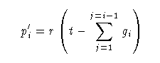
If within a group defined for the function Combine the distributions are given a Gap gi then the combination is performed as:
We can then define a new set of original distributions p'i using
p'i = r(t+gi)
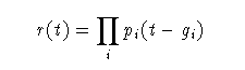
A very similar method to this is used for wiggle matching using the command D_Sequence, only difference being the way in which the gap is defined (between each successive distribution). A probability distribution r(t) is always calculated for the start of the sequence. This is given by:

and the resultant distributions then calculated using:
In the case of Bayesian wiggle matches and combinations, the program also calculates the chi-squared value for the best fit (ie the highest point on the probability distribution). This is reported in the text log file. For wiggle matching tree ring sequences, where the overall precision can be very high, you use a resolution of one year.
See also [Archaeological Considerations]

and so if a group of events are independent the probability of being after all of them is given by:

This is the distribution (normalised to a maximum of 1) returned by After. From this a distribution r'(t) can be calculated which gives a probability distribution for the last of the group of events:
r'(t) = dr(t)/dt
This is the distribution returned by the request Last within a phase if MCMC sampling is not needed.
The probabilities of being before a group of events and a distribution for the first event of a phase can be similarly defined.
WARNING: These methods assume that the events are entirely independant; in most cases a much better estimate will be arrived at using MCMC sampling from a phase which is enclosed within Boundary events.
See also [Archaeological Considerations]
r(t) = p(t-dt)
If the offset has an error associated with it then dt+-sigma the distribution is given by:

A similar method is used to calculate a probability distribution for the age difference between two independent distributions (only employed when MCMC sampling is not necessary) using Difference.

And to shift one distribution by another using Shift:

See also [Archaeological Considerations]